38 how to add data labels to a pie chart in excel on mac

How to insert data labels to a Pie chart in Excel 2013 - YouTube This video will show you the simple steps to insert Data Labels in a pie chart in Microsoft® Excel 2013. Content in this video is provided on an "as is" basi... Adding Data Labels to Your Chart - Excel ribbon tips Select the position that best fits where you want your labels to appear. To add data labels in Excel 2013 or later versions, follow these steps: Activate the chart by clicking on it, if necessary. Make sure the Design tab of the ribbon is displayed. (This will appear when the chart is selected.) Click the Add Chart Element drop-down list.

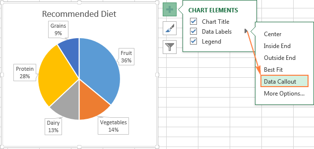
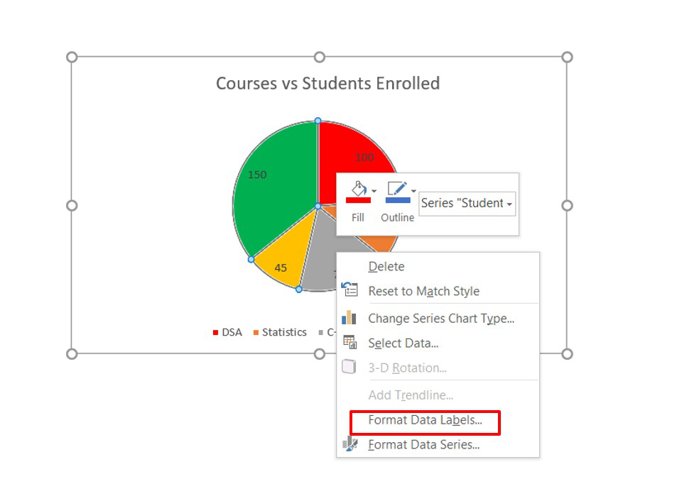
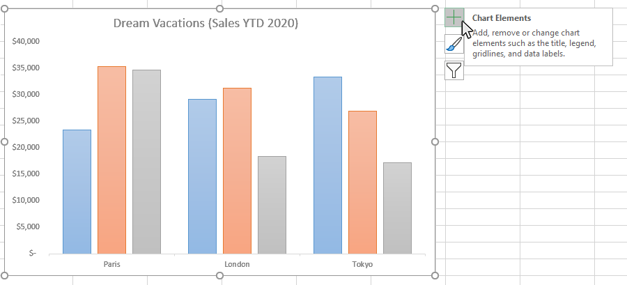
How to Make a Pie Chart with Multiple Data in Excel (2 Ways) - ExcelDemy First, to add Data Labels, click on the Plus sign as marked in the following picture. After that, check the box of Data Labels. At this stage, you will be able to see that all of your data has labels now. Next, right-click on any of the labels and select Format Data Labels. After that, a new dialogue box named Format Data Labels will pop up.

How to add data labels to a pie chart in excel on mac

How To Add Text To A Pie Chart In Excel For Mac To display percentage values as labels on a pie chart. Add a pie chart to your report. For more information, see Add a Chart to a Report (Report Builder and SSRS). On the design surface, right-click on the pie and select Show Data Labels. The data labels should appear within each slice on the pie chart. Office: Display Data Labels in a Pie Chart - Tech-Recipes: A Cookbook ... 2. If you have not inserted a chart yet, go to the Insert tab on the ribbon, and click the Chart option. 3. In the Chart window, choose the Pie chart option from the list on the left. Next, choose the type of pie chart you want on the right side. 4. Once the chart is inserted into the document, you will notice that there are no data labels. Add data labels and callouts to charts in Excel 365 - EasyTweaks.com Step #2: When you select the "Add Labels" option, all the different portions of the chart will automatically take on the corresponding values in the table that you used to generate the chart. The values in your chat labels are dynamic and will automatically change when the source value in the table changes. Step #3: Format the data labels.

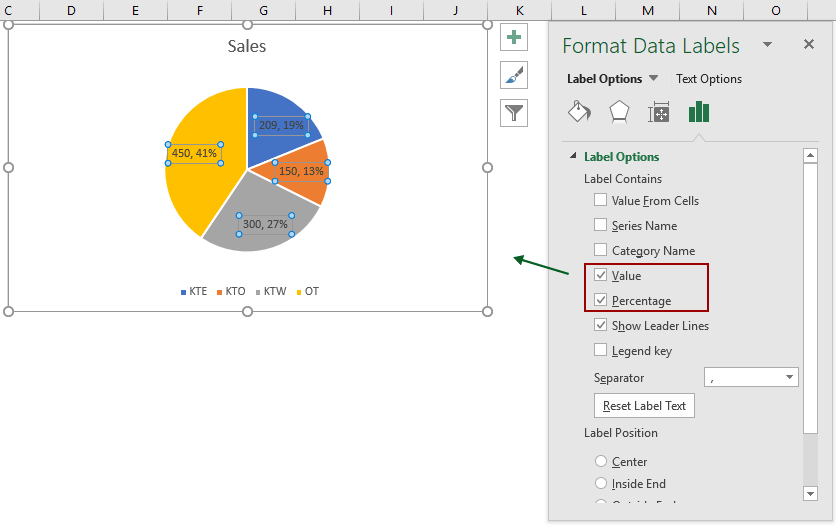
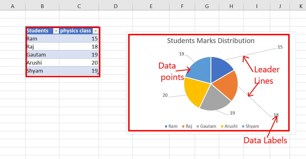
How to add data labels to a pie chart in excel on mac. How to display leader lines in pie chart in Excel? - ExtendOffice To display leader lines in pie chart, you just need to check an option then drag the labels out. 1. Click at the chart, and right click to select Format Data Labels from context menu. 2. In the popping Format Data Labels dialog/pane, check Show Leader Lines in the Label Options section. See screenshot: 3. Adding Data Labels to Charts/Graphs in Excel - AdvantEdge Training ... First Method -. In the Design tab of the Chart Tools contextual tab, go to the Chart Layouts group on the far left side of the ribbon, and click Add Chart Element. In the drop-down menu, hover on Data Labels. This will cause a second drop-down menu to appear. Choose Outside End for now and note how it adds labels to the end of each pie portion. Pie Chart in Excel | How to Create Pie Chart - EDUCBA Go to the Insert tab and click on a PIE. Step 2: once you click on a 2-D Pie chart, it will insert the blank chart as shown in the below image. Step 3: Right-click on the chart and choose Select Data. Step 4: once you click on Select Data, it will open the below box. Step 5: Now click on the Add button. it will open the below box. Change the format of data labels in a chart To get there, after adding your data labels, select the data label to format, and then click Chart Elements > Data Labels > More Options. To go to the appropriate area, click one of the four icons ( Fill & Line, Effects, Size & Properties ( Layout & Properties in Outlook or Word), or Label Options) shown here.

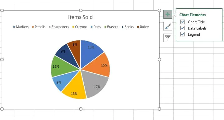
Adding data labels to a Pie Chart in VBA - Automate Excel VBA Code Examples for Excel. Excel. Formula Tutorials; Excel Functions List with Examples (Free Downloads!) Excel Formulas Examples List. Excel Boot Camp. Shortcuts. Shortcut Training App; List of Shortcuts; Shortcut Coach. Charts. Chart Templates; Chart Add-in; Charts List; Excel VBA Consulting - Get Help & Hire an Expert! c# - Add data labels to excel pie chart - Stack Overflow I am drawing a pie chart with some data: private void DrawFractionChart(Excel.Worksheet activeSheet, Excel.ChartObjects xlCharts, Excel.Range xRange, Excel.Range yRange) { Excel.ChartObject ... Add data labels to excel pie chart. Ask Question Asked 10 years, 1 month ago. Modified 6 years, 2 months ago. Viewed 9k times ... Why is a virtual MAC ... How to add axis labels in Excel Mac - Quora Add a chart title 1. In the chart, select the "Chart Title" box and type in a title. 2. Select the + sign to the top-right of the chart. 3. Select the arrow next to Chart Title. 4. Select Centered Continue Reading Reclusive Roy 1 y Related How do I move rows in Excel on a Mac? Take your cursor to the row no. and press it. Microsoft Excel Tutorials: Add Data Labels to a Pie Chart - Home and Learn You should get the following menu: From the menu, select Add Data Labels. New data labels will then appear on your chart: The values are in percentages in Excel 2007, however. To change this, right click your chart again. From the menu, select Format Data Labels: When you click Format Data Labels , you should get a dialogue box. This one:

Excel custom pie chart labels - Microsoft Community Answer HansV MVP MVP Replied on July 8, 2019 Specify (space) as Separator in the Data Labels. Set the Number format of the data labels to Custom, and specify (0%) as Type. --- Kind regards, HansV Report abuse 6 people found this reply helpful · Was this reply helpful? Yes No Pie chart in Excel with data labels instead of hard to read legend 00:00 create pie chart in excel 00:13 remove legend from a chart 00:18 add labels to each slice in a pie chart 00:29 change chart labels to show description and % rather then number 00:58 place all... How to add data labels from different column in an Excel chart? Please do as follows: 1. Right click the data series in the chart, and select Add Data Labels > Add Data Labels from the context menu to add data labels. 2. Right click the data series, and select Format Data Labels from the context menu. 3. Adding data labels to a pie chart - Excel General - OzGrid Free Excel ... Re: Adding data labels to a pie chart Yes it doesn't appear via intelli-sense unless you use a Series object. Code Dim objSeries As Series Set objSeries = ActiveChart.SeriesCollection (1) objSeries.HasDataLabels [h4] Cheers Andy [/h4] norie Super Moderator Reactions Received 8 Points 53,548 Posts 10,650 Feb 25th 2005 #9

How to show percentage in pie chart in Excel?

How Do I Add A Pie Chart In Excel For Mac - herevload Excel charts allow you to do a lot of customizations that help in representing the data in the best possible way. And one such example of customization is the ease with which you can add a secondary...

Excel for Mac: Getting Started with Charts

Add or remove data labels in a chart - support.microsoft.com Click the data series or chart. To label one data point, after clicking the series, click that data point. In the upper right corner, next to the chart, click Add Chart Element > Data Labels. To change the location, click the arrow, and choose an option. If you want to show your data label inside a text bubble shape, click Data Callout.

How to make a pie chart in Excel

How to add data labels in excel to graph or chart (Step-by-Step) Add data labels to a chart 1. Select a data series or a graph. After picking the series, click the data point you want to label. 2. Click Add Chart Element Chart Elements button > Data Labels in the upper right corner, close to the chart. 3. Click the arrow and select an option to modify the location. 4.

microsoft excel - How do I reposition data labels with a ...

Change the look of chart text and labels in Numbers on Mac Click the chart to change all item labels, or click one item label to change it. To change several item labels, Command-click them. In the Format sidebar, click the Wedges or Segments tab. To add labels, do any of the following: Show data labels: Select the checkbox next to Data Point Names. Show data values: Select the checkbox next to Values.

How to Show Percentage in Pie Chart in Excel? - GeeksforGeeks

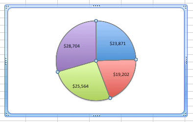
Create A Pie Chart In Excel With and Easy Step-By-Step Guide However, it is recommended that you add the actual values from the dataset to every slice of the pie chart. They are known as data labels. If you want to add the data labels then follow these steps: Step 1: Right-click on any of the slices. Step 2: Click on "Add data labels". This will add values to every slice in the pie chart in Excel.

How to Make a Pie Chart in Excel - All Things How

How to Create and Format a Pie Chart in Excel - Lifewire To add data labels to a pie chart: Select the plot area of the pie chart. Right-click the chart. Select Add Data Labels . Select Add Data Labels. In this example, the sales for each cookie is added to the slices of the pie chart. Change Colors

How to Make a Pie Chart in Excel 2010, 2013, 2016?

Formatting data labels and printing pie ... - Microsoft Community Here's a work around I found for printing pie charts. Still can't find a solution for formatting the data labels. 1. When printing a pie chart from Excel for mac 2019, MS instructions are to select the chart only, on the worksheet > file > print. Excel is supposed to print the chart only (not the data ) and automatically fit it onto one page.

Change the format of data labels in a chart

Add or remove data labels in a chart - Microsoft Support This displays the Chart Tools, adding the Design, and Format tabs. On the Design tab, in the Chart Layouts group, click Add Chart Element, choose Data Labels, and then click None. Click a data label one time to select all data labels in a data series or two times to select just one data label that you want to delete, and then press DELETE.

microsoft excel 2016 - How do I move the legend position in a ...

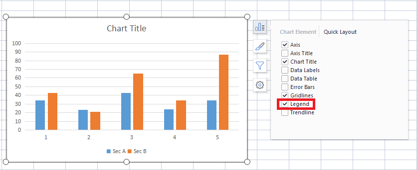
Create a Pie Chart in Excel (In Easy Steps) - Excel Easy Create the pie chart (repeat steps 2-3). 7. Click the legend at the bottom and press Delete. 8. Select the pie chart. 9. Click the + button on the right side of the chart and click the check box next to Data Labels. 10. Click the paintbrush icon on the right side of the chart and change the color scheme of the pie chart.

How to Add Data Tables to a Chart in Excel - Business ...

How to Make a Pie Chart in Excel & Add Rich Data Labels to The Chart! Here we will combine this two errors in a pie chart. So let`s start the procedure. The source data is shown below: Creating and formatting the Pie Chart 1) Select the data. 2) Go to Insert> Charts> click on the drop-down arrow next to Pie Chart and under 2-D Pie, select the Pie Chart, shown below.

How to make a pie chart in Excel

Add data labels and callouts to charts in Excel 365 - EasyTweaks.com Step #2: When you select the "Add Labels" option, all the different portions of the chart will automatically take on the corresponding values in the table that you used to generate the chart. The values in your chat labels are dynamic and will automatically change when the source value in the table changes. Step #3: Format the data labels.

How to Add Leader Lines in Excel? - GeeksforGeeks

Office: Display Data Labels in a Pie Chart - Tech-Recipes: A Cookbook ... 2. If you have not inserted a chart yet, go to the Insert tab on the ribbon, and click the Chart option. 3. In the Chart window, choose the Pie chart option from the list on the left. Next, choose the type of pie chart you want on the right side. 4. Once the chart is inserted into the document, you will notice that there are no data labels.