43 how to add custom data labels in excel

Add Custom Labels to x-y Scatter plot in Excel ... Step 1: Select the Data, INSERT -> Recommended Charts -> Scatter chart (3 rd chart will be scatter chart) Let the plotted scatter chart be Step 2: Click the + symbol and add data labels by clicking it as shown below Step 3: Now we need to add the flavor names to the label.Now right click on the label and click format data labels. Under LABEL OPTIONS select Value From Cells as shown below. Format Data Labels in Excel- Instructions - TeachUcomp, Inc. To do this, click the "Format" tab within the "Chart Tools" contextual tab in the Ribbon. Then select the data labels to format from the "Chart Elements" drop-down in the "Current Selection" button group. Then click the "Format Selection" button that appears below the drop-down menu in the same area.

Apply Custom Data Labels to Charted Points - Peltier Tech Click once on a label to select the series of labels. Click again on a label to select just that specific label. Double click on the label to highlight the text of the label, or just click once to insert the cursor into the existing text. Type the text you want to display in the label, and press the Enter key.

How to add custom data labels in excel

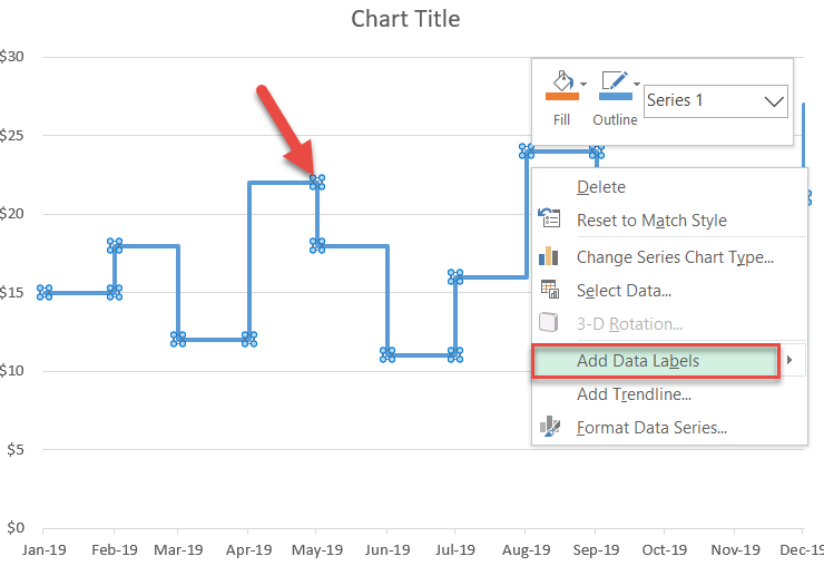
How to add data labels from different column in an Excel ... Right click the data series in the chart, and select Add Data Labels > Add Data Labels from the context menu to add data labels. 2. Click any data label to select all data labels, and then click the specified data label to select it only in the chart. 3. Custom Data Labels with Colors and Symbols in Excel Charts ... To apply custom format on data labels inside charts via custom number formatting, the data labels must be based on values. You have several options like series name, value from cells, category name. But it has to be values otherwise colors won't appear. Symbols issue is quite beyond me. › blog › how-to-make-ahow to make a scatter plot in Excel — storytelling with data Feb 02, 2022 · To add data labels to a scatter plot, just right-click on any point in the data series you want to add labels to, and then select “Add Data Labels…” Excel will open up the “Format Data Labels” pane and apply its default settings, which are to show the current Y value as the label. (It will turn on “Show Leader Lines,” which I ...

How to add custom data labels in excel. Excel charts: add title, customize chart axis, legend and ... Depending on where you want to focus your users' attention, you can add labels to one data series, all the series, or individual data points. Click the data series you want to label. To add a label to one data point, click that data point after selecting the series. Click the Chart Elements button, and select the Data Labels option. How to Print Labels from Excel - Lifewire Select Mailings > Write & Insert Fields > Update Labels . Once you have the Excel spreadsheet and the Word document set up, you can merge the information and print your labels. Click Finish & Merge in the Finish group on the Mailings tab. Click Edit Individual Documents to preview how your printed labels will appear. Select All > OK . Improve your X Y Scatter Chart with custom data labels Press with right mouse button on on a chart dot and press with left mouse button on on "Add Data Labels" Press with right mouse button on on any dot again and press with left mouse button on "Format Data Labels" A new window appears to the right, deselect X and Y Value. Enable "Value from cells" Select cell range D3:D11 How to Customize Your Excel Pivot Chart Data Labels - dummies To add data labels, just select the command that corresponds to the location you want. To remove the labels, select the None command. If you want to specify what Excel should use for the data label, choose the More Data Labels Options command from the Data Labels menu. Excel displays the Format Data Labels pane.

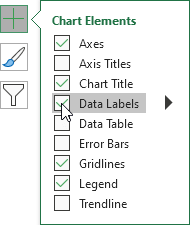
How to add or move data labels in Excel chart? To add or move data labels in a chart, you can do as below steps: In Excel 2013 or 2016. 1. Click the chart to show the Chart Elements button . 2. Then click the Chart Elements, and check Data Labels, then you can click the arrow to choose an option about the data labels in the sub menu. See screenshot: In Excel 2010 or 2007 chandoo.org › wp › change-data-labels-in-chartsHow to Change Excel Chart Data Labels to Custom Values? May 05, 2010 · First add data labels to the chart (Layout Ribbon > Data Labels) Define the new data label values in a bunch of cells, like this: Now, click on any data label. This will select “all” data labels. Now click once again. At this point excel will select only one data label. Add / Move Data Labels in Charts - Excel & Google Sheets ... Adding Data Labels Click on the graph Select + Sign in the top right of the graph Check Data Labels Change Position of Data Labels Click on the arrow next to Data Labels to change the position of where the labels are in relation to the bar chart Final Graph with Data Labels Add or remove data labels in a chart To label one data point, after clicking the series, click that data point. In the upper right corner, next to the chart, click Add Chart Element > Data Labels. To change the location, click the arrow, and choose an option. If you want to show your data label inside a text bubble shape, click Data Callout.

Custom Chart Data Labels In Excel With Formulas Follow the steps below to create the custom data labels. Select the chart label you want to change. In the formula-bar hit = (equals), select the cell reference containing your chart label's data. In this case, the first label is in cell E2. Finally, repeat for all your chart laebls. support.microsoft.com › en-us › officeCreate a diagram in Excel with the Visio Data Visualizer add-in The Data Visualizer add-in is available for Excel on PC, Mac, and the browser with a Microsoft 365 work or school account. (If the only Microsoft account you have is a personal one—that is, hotmail.com, live.com, outlook.com, or msn.com—you can still try out parts of the Data Visualizer add-in without signing in. Make your Excel charts easier to read with custom data labels Make your Excel charts easier to read with custom data labels . If users are spending time trying to match up each data label in your chart with its corresponding data point, then you may need to ... How to create Custom Data Labels in Excel Charts Two ways to do it. Click on the Plus sign next to the chart and choose the Data Labels option. We do NOT want the data to be shown. To customize it, click on the arrow next to Data Labels and choose More Options … Unselect the Value option and select the Value from Cells option. Choose the third column (without the heading) as the range.

Enable or Disable Excel Data Labels at the click of a button - How To - PakAccountants.com

Excel tutorial: How to use data labels Generally, the easiest way to show data labels to use the chart elements menu. When you check the box, you'll see data labels appear in the chart. If you have more than one data series, you can select a series first, then turn on data labels for that series only. You can even select a single bar, and show just one data label. In a bar or column ...

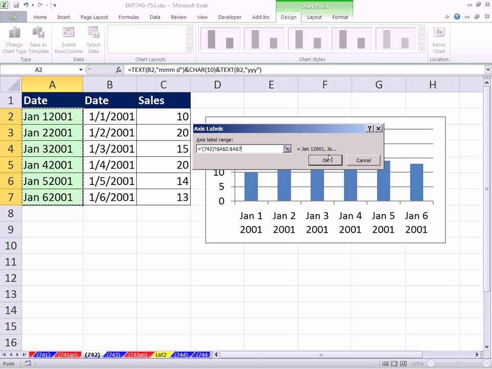
Excel Magic Trick 742: Wrap Text In Chart Label Using CHAR function and Code 10 - YouTube

Custom data labels in a chart - Get Digital Help Add data labels Press with right mouse button on on a column Press with left mouse button on "Add Data Labels" Double press with left mouse button on a data label Deselect Value Select Category name Press with left mouse button on Close Get the Excel file Custom-data-labels-in-a-chartv3.xlsx Weekly Blog EMAIL [newsletter_signup_form id=1] Welcome!

How to Import Excel Data into a Label File in Custom Designer | Brady Support

Adding rich data labels to charts in Excel 2013 ... The data labels up to this point have used numbers and text for emphasis. Putting a data label into a shape can add another type of visual emphasis. To add a data label in a shape, select the data point of interest, then right-click it to pull up the context menu. Click Add Data Label, then click Add Data Callout. The result is that your data ...

Adobe Acrobat Standard Help 7.0 Instruction Manual 7 En

Add or remove data labels in a chart To label one data point, after clicking the series, click that data point. In the upper right corner, next to the chart, click Add Chart Element > Data Labels. To change the location, click the arrow, and choose an option. If you want to show your data label inside a text bubble shape, click Data Callout.

Excel 2013 Tutorial Formatting Data Labels Microsoft Training Lesson 28.6 - YouTube

› charts › axis-labelsHow to add Axis Labels (X & Y) in Excel & Google Sheets ... Excel offers several different charts and graphs to show your data. In this example, we are going to show a line graph that shows revenue for a company over a five-year period. In the below example, you can see how essential labels are because in this below graph, the user would have trouble understanding the amount of revenue over this period.

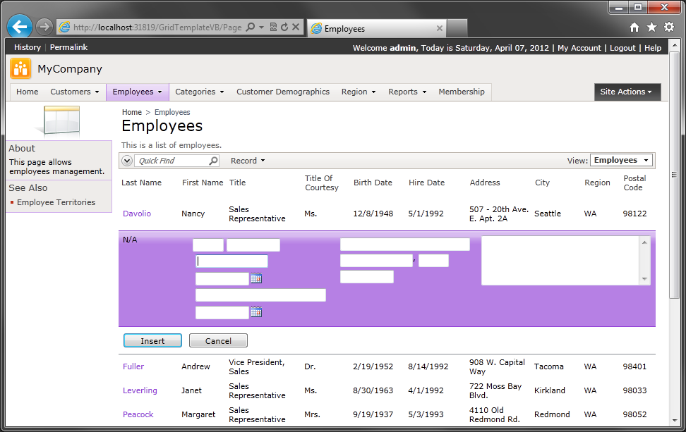
Code On Time: User Interface / Grid Templates / Grid Template for 'New' Mode

how to add data labels into Excel graphs — storytelling ... The data labels for the two lines are not, technically, "data labels" at all. A text box was added to this graph, and then the numbers and category labels were simply typed in manually. This is what we affectionately refer to as "brute-forcing" your tool to make it look the way you want it to, regardless of its defaults.

Enable or Disable Excel Data Labels at the click of a button - How To - PakAccountants.com

How to Use Cell Values for Excel Chart Labels Select the chart, choose the "Chart Elements" option, click the "Data Labels" arrow, and then "More Options.". Uncheck the "Value" box and check the "Value From Cells" box. Select cells C2:C6 to use for the data label range and then click the "OK" button. The values from these cells are now used for the chart data labels.

Format Data Labels in Excel- Instructions - TeachUcomp, Inc.

Excel tutorial: How to customize axis labels Instead you'll need to open up the Select Data window. Here you'll see the horizontal axis labels listed on the right. Click the edit button to access the label range. It's not obvious, but you can type arbitrary labels separated with commas in this field. So I can just enter A through F. When I click OK, the chart is updated.

How-to Use Data Labels from a Range in an Excel Chart - Excel Dashboard Templates

support.microsoft.com › en-us › officeEdit titles or data labels in a chart - support.microsoft.com You can also place data labels in a standard position relative to their data markers. Depending on the chart type, you can choose from a variety of positioning options. On a chart, do one of the following: To reposition all data labels for an entire data series, click a data label once to select the data series.

How to Create an Excel Box Plot - Complete tutorial

Using the CONCAT function to create custom data labels for ... Use the chart skittle (the "+" sign to the right of the chart) to select Data Labels and select More Options to display the Data Labels task pane. Check the Value From Cells checkbox and select the cells containing the custom labels, cells C5 to C16 in this example.

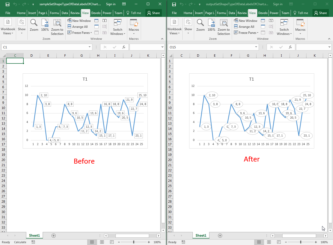
Set the Shape Type of Data Labels of Chart | Documentation

Adding Data Labels to Your Chart (Microsoft Excel) To add data labels in Excel 2013 or Excel 2016, follow these steps: Activate the chart by clicking on it, if necessary. Make sure the Design tab of the ribbon is displayed. (This will appear when the chart is selected.) Click the Add Chart Element drop-down list. Select the Data Labels tool.

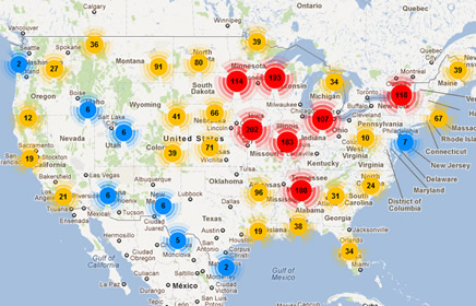
Create marker clustering maps

Adding Data Labels To An Excel Chart | MyExcelOnline In our example below, I add a Data Label to a column chart and then I format the data label using CTRL+1. I then select to custom format the numbers so it shows the values as thousands by adding a comma , after each zero and then showing the work k by adding "k". Example Custom Number Format: [$$-1004]#,##0 ,"k" ;- [$$-1004]#,##0 ,"k".

Excel Dual Axis on same side - Super User

Add a DATA LABEL to ONE POINT on a ... - Excel Quick Help Steps shown in the video above: Click on the chart line to add the data point to. All the data points will be highlighted. Click again on the single point that you want to add a data label to. Right-click and select ' Add data label ' This is the key step! Right-click again on the data point itself (not the label) and select ' Format data label '.

Create Charts in Excel - Easy Excel Tutorial

How to Add Data Labels to an Excel 2010 Chart - dummies Excel provides several options for the placement and formatting of data labels. Use the following steps to add data labels to series in a chart: Click anywhere on the chart that you want to modify. On the Chart Tools Layout tab, click the Data Labels button in the Labels group. A menu of data label placement options appears: None: The default ...

How to Create a Step Chart in Excel - Automate Excel

› blog › how-to-make-ahow to make a scatter plot in Excel — storytelling with data Feb 02, 2022 · To add data labels to a scatter plot, just right-click on any point in the data series you want to add labels to, and then select “Add Data Labels…” Excel will open up the “Format Data Labels” pane and apply its default settings, which are to show the current Y value as the label. (It will turn on “Show Leader Lines,” which I ...

Format Data Labels in Excel- Instructions - TeachUcomp, Inc.

Custom Data Labels with Colors and Symbols in Excel Charts ... To apply custom format on data labels inside charts via custom number formatting, the data labels must be based on values. You have several options like series name, value from cells, category name. But it has to be values otherwise colors won't appear. Symbols issue is quite beyond me.